This online appendix supports the MEng Project 'Optimal Siting of Energy Storage in Fully Renewable Power Grids', available for download here. It provides details of the data sources, data preparation methodology, and code listings for the dual optimisation and solution recovery implementations used in the numerical experiments performed, which are discussed in Section V of the report. It also presents some 'back of the envelope' calculations which motivate the development of formulations of the renewable power system optimisation problem which account for full complexity, non-linear line losses.
Data sources
In order to provide a reasonable representation of the diversity of renewable generation assets expected in future power systems, the historic bus generation power time series required
for the optimisation method were synthesised from meterological observation data. This data was obtained from the MetOffice's MIDAS dataset [A1]. Offshore wind speed measurements were
used to estimate historic offshore wind generation potential, and onshore 'cloudiness' measurements were used to estimate historic solar generation potential.
Fig. A1 shows the locations of the MET MIDAS measurement stations selected for use in the data synthesis, alongside the simplified model of the UK transmission level power
system used in the experiments. Additionally, the geographic clustering of measurement data to system model buses is indicated by colouring of the measurement station markers.
Fig. A2 shows the location of all available MET MIDAS marine measurement stations providing wind speed data (blue), and onshore measurement stations
providing cloudiness data (green).
Historic electricity demand data for the UK was obtained from the GridWatch dataset [A2].
Data preparation methodology
Generation
The meterological observation data for each measurement station for each data type was pre-processed prior to the data synthesis. The available set of measurement stations was screened, with only those with valid locations (i.e. both within the UK and consistent with the data type) and more than 6 months of data availability were selected. The observation time series for each valid measurement station were then resampled/interpolated to match the 'on the hour' timestamps used as the common sampling times for all data time series. Finally, measurement stations were assigned to nodes in the transmission network model by geographical proximity.
Wind
The wind power generation time series for each bus in the transmission network model were synthesised from the wind speed measurement time series of the assigned measurement stations as follows.
At each time instance, the measurement stations with available wind speed measurements were identified. For each of these stations, the wind speed measurement was sheared from the assumed average
measurement height of 10m, to the chosen characteristic offshore wind turbine hub height of 150m, using the power law wind speed extrapolation model,
$$v_2 = v_1 \cdot \left(\frac{z_2}{z_1}\right)^{\alpha}$$
with a shear exponent of \(\alpha=0.11\), which is typical for offshore conditions [A3].
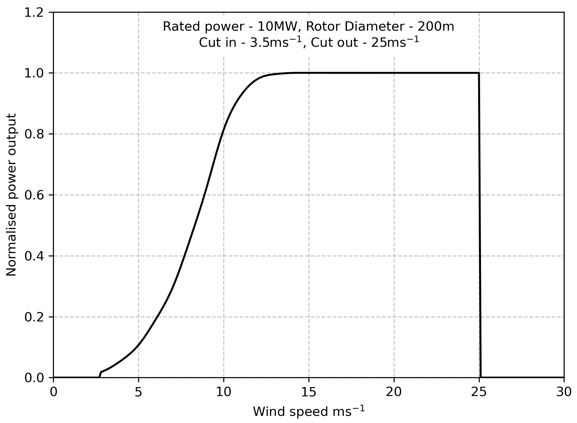
These sheared wind speed values were then converted to normalised wind turbine power output values, using the power curve shown in Fig. A3. This power curve was generated from the parametric
wind turbine power curve model from [A4], assuming \(10\:MW\) turbines with \(200\:m\) rotor diameters, and cut-in and cut-out speeds of \(3.5\:ms^{-1}\) and \(25\:ms^{-1}\) respectively. These parameter values were
chosen to represent next-generation, high power offshore wind turbines, to provide a better approximation of future wind generation behaviour.
The average of the normalised output powers over the available measurements was then taken to give the normalised wind power generation value for that bus. At evaluation time, these values were
multiplied by the installed wind capacity at the bus to yield the synthesised wind power generation values.
Solar
The solar power generation time series for each bus in the transmission network model were synthesised from the 'cloudiness' measurement time series of the assigned measurement stations as follows.
For each day, the average 'cloudiness' factor over the daylight hours was determined for each measurement station with available data. The average of the available daily 'cloudiness' values was
then taken to represent the average cloud cover at that node on that day. The daily average 'cloudiness' values were used as the hourly measurements were found to be excessively noisy, and the resulting synthesised
data did not match the true solar generation measurements from GridWatch [A2].
These daily 'cloudiness' factors were then converted to power output reduction factors for solar generation using an empirical model from [A5], shown in Fig. A4.
Solar power output time series were synthesised using the solarpy [A6] Python module. This module computes the theoretical solar power generation
of a panel at a given location (latitude) at a given time. This was used to calculate approximate solar generation powers at each node location at each sampling time instace, which were the normalised by the
maximum solar generation power over all nodes over all times.
Finally, the normalised generation values were modulated/multiplied by the corresponding daily power output reduction factors to incorporate the weather observation data into the sythesised solar generation
time series. Again, at evaluation time, the normalised values were multiplied by the installed solar generation capacity at the bus to yield the synthesised solar power generation values.

Demand
GridWatch [A2] provides historic UK electricity demand data. This data was cleaned and resampled to the 'on the hour' timestamps. The bus demand power time series were then produced by scaling the instantaneous national demand power values by a factor representing the fraction of the UK's population served by each bus. These factors are defined as part of the transmission network model, see test_net.py.
Network
The simplified model the UK transmission level power system, shown in Fig. A1 & Fig. 1 of the report, was based off a map of the European power grid published by the European Network of Transmission System Operators for Electricity (ENTSO-E) [A7].
Renewable Generation & Demand Power Time Series
Fig. A5 plots the normalised wind, solar, and demand power time series produced, averaged over all buses. A plot of the bus power time series used in the numerical experiments is available
here.
Motivating 'Back of the Envelope' Calculations
The following two calculations motivate the development of renewable power system optimisation tools which account for the full complexity power network physics. The first demonstrating the substantial impact that line losses may have on the operation of a future, fully renewable UK power system, and the second, the scale of the potential savings which true optimal power system infrastructure development strategies could provide.
Power Losses
Assume high voltage transmission lines to have a nominal voltage of \(400\:kV\) and a line impedance of \((25+\mathbf{j}210)\:m\Omega/km\) [A8,A9].
Consider a scenario in which, at some time instance, there is little renewable generation in the South East, and power must be transmitted from
Scotland to fulfil demand. Assume that power is transmitted from Edinburgh to fulfil \(1\:GW\) of demand in London. This results in a transmission
distance of \(\approx 500\:km\). A transmission line of this length has a resistance of \(12.5\:\Omega .\)
For \(1\:GW\) of power to be recieved in London, the transmission current must be,
$$I = \frac{P}{V_{\text{nom}}} = \frac{1GW}{400kV} = 2.5\:kA$$
and so the incurred real power transmission loss is,
$$I^2 R = (2.5 \times 10^3)^2 \times 12.5 = 78.125\:MW$$
Therefore, the power transmission loss is roughly 10% of the recieved energy, even when the contribution of reactive power to line current is neglected.
Due to the quadratic nature of line losses, the proportion of recieved energy lost in transmission in this scenario increases linearly with the recieved power,
$$\text{% P lost} = \frac{I^2 R}{P_{\text{rec}}} = \frac{I^2 R}{IV_{\text{nom}}} = \frac{IR}{V_{\text{nom}}} = \frac{\Delta V}{V_{\text{nom}}}$$
However, a linearised power flow model is unable to capture this varying loss contribution.
When the required recieved power increases to \(5\:GW\), the transmission loss of \(1.95\:GW\) makes up \(\approx 40\%\) of the recieved power, or \(\approx 30\%\)
of the generated power. Hence, in this scenario, it becomes a critical determinant of the overall system efficiency, and thus plays a significant role in the
cost of electricity provision.
Therefore, system operation strategies which account for this full complexity loss information may be able to provide substantially improved system performance,
and so reduce the overall cost of supporting renewable electricity generaiton in power systems.
Note for comparison, that at present the UK peak electricity demand is \(\approx 60\:GW\) [A2], and roughly \(13\%\) of the UK's population lives in Greater London.
Therefore, London's peak electricity demand is approximately \(8\:GW\), and so the assumption of \(5\:GW\) of recieved power is not unreasonable.
System Cost of Electricity Provision
In 2019, the UK's total energy consumption was \(1650\:TWh\) [A10], of which \(346\:TWh\) was electricity consumption [A11] (including energy industry usage and system losses).
Assume the 2018/19 average wholesale day-ahead price, of \(£ 58.6/MWh\) [A12], to be a reasonable lower bound estimate of the current value of electricity. This results
in the lower bound estimate of the current value of UK electricity consumption to be \(£ 20.3bn/yr\).
Following substantial electrification of the heating and transportation sector, a conservative estimate of total electricity consumption in the UK would be of the order
\(1000\:TWh/yr\). Assume an increase in the lower bound unit cost of electricity provision to \(£ 75/MWh\) [A13,A14], to account for the higher cost of renewable generation, and
the additional system operation costs associated with supporting variable renewable sources, such as energy storage and reactive power support.
This yields a long term lower bound estimate of the overall cost of providing fully renewable energy in the UK of \(£ 75bn/yr\). Hence, if a renewable power systems
optimisation method is able to determine a more cost effective system development strategy which provides only slightly over a percentage point reduction in cost, this
amounts to a cost saving to the consumer of the order \(£ 1bn/yr\).
For comparison, the in tax year 2018/19, the NHS cost \(£ 152.9bn\) to run.
Code Listings for Optimisation Implementation
Code listings for a Python-based implementation of the formulated optimisation and solution strategies in Section IV of the report, and the definition of the test network used in the numerical experiments in Section V of the report, are provided in the following files respectively:
Note to examiners
Whilst this online appendix provides supporting material for the IIB Project report entitled 'Optimal Siting of Energy Storage in Fully Renewable Power Grids', it is not submitted formally for consideration as part of that report, and is provided purely as reference material and a host for interactive figures and code listings.